example CDReSp

Calculate constant ductility response spectra in OpenSeismoMatlab

Earthquake motion
Setup parameters for CDReSp function
Calculate spectra and pseudospectra
Plot the spectra
Copyright

Earthquake motion

For reproducibility

rng(0)

Generate earthquake data

dt=0.02;
N=10;
a=rand(N,1)-0.5;
b=100*pi*rand(N,1);
c=pi*(rand(N,1)-0.5);
t=(0:dt:(100*dt))';
xgtt=zeros(size(t));
for i=1:N
    xgtt=xgtt+a(i)*sin(b(i)*t+c(i));
end

Setup parameters for CDReSp function

Eigenperiods

T=(0.04:0.04:4)';

Critical damping ratio

ksi=0.05;

Ductility

mu=2;

Maximum number of iterations

n=50;

Tolerance for convergence to target ductility

tol=0.01;

Post-yield stiffness factor

pysf=0.1;

Maximum ratio of the integration time step to the eigenperiod

dtTol=0.02;

Algorithm to be used for the time integration

AlgID='U0-V0-Opt';

Minimum absolute value of the eigenvalues of the amplification matrix

rinf=1;

Maximum tolerance of convergence for time integration algorithm

maxtol=0.01;

Maximum number of iterations per integration time step

jmax=200;

Infinitesimal acceleration

dak=eps;

Calculate spectra and pseudospectra

Apply CDReSp

[CDPSa,CDPSv,CDSd,CDSv,CDSa,fyK,muK,iterK]=CDReSp(dt,xgtt,T,ksi,...
    mu,n,tol,pysf,dtTol,AlgID,rinf,maxtol,jmax,dak);

Plot the spectra

Constant ductility displacement spectrum

figure()
plot(T,CDSd,'k','LineWidth',1)
ylabel('Spectral displacement (m)')
xlabel('Eigenperiod (sec)')
drawnow;
pause(0.1)

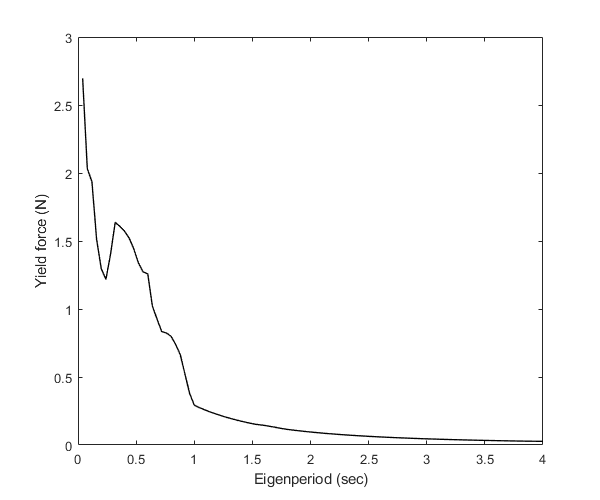
Constant ductility yield force spectrum

figure()
plot(T,fyK,'k','LineWidth',1)
ylabel('Yield force (N)')
xlabel('Eigenperiod (sec)')
drawnow;
pause(0.1)

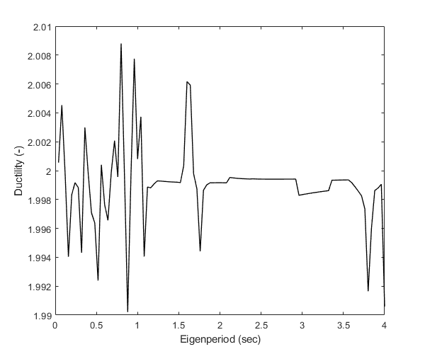
Achieved ductility

figure()
plot(T,muK,'k','LineWidth',1)
ylabel('Ductility (-)')
xlabel('Eigenperiod (sec)')
drawnow;
pause(0.1)

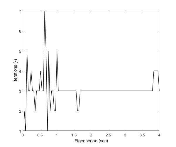
Iterations

figure()
plot(T,iterK,'k','LineWidth',1)
ylabel('Iterations (-)')
xlabel('Eigenperiod (sec)')
drawnow;
pause(0.1)

Copyright