example LEReSp

Calculate linear elastic response spectra in OpenSeismoMatlab

Contents

Generate earthquake motion

For reproducibility

rng(0)

Generate earthquake acceleration time history

dt=0.02;
N=10;
a=rand(N,1)-0.5;
b=100*pi*rand(N,1);
c=pi*(rand(N,1)-0.5);
t=(0:dt:(100*dt))';
xgtt=zeros(size(t));
for i=1:N
    xgtt=xgtt+a(i)*sin(b(i)*t+c(i));
end

Plot the generated time history

figure()
plot(t,xgtt,'k','LineWidth',1)
ylabel('Acceleration (m/s^2)')
xlabel('Time (sec)')
title('Artificial acceleration time history')
drawnow;
pause(0.1)

Setup parameters for LEReSp function

Eigenperiods

T=logspace(log10(0.02),log10(5),1000)';

Critical damping ratio

ksi=0.05;

Maximum ratio of the integration time step to the eigenperiod

dtTol=0.02;

Algorithm to be used for the time integration

AlgID='U0-V0-Opt';

Minimum absolute value of the eigenvalues of the amplification matrix

rinf=1;

Calculate spectra and pseudospectra

Apply LEReSp

[PSa,PSv,Sd,Sv,Sa,Siev]=LEReSp(dt,xgtt,T,ksi,dtTol,AlgID,rinf);

Plot the spectra and pseudospectra

Pseudoacceleration spectrum

figure()
plot(T,PSa,'k','LineWidth',1)
ylabel('Pseudoacceleration (m/s^2)')
xlabel('Eigenperiod (sec)')
drawnow;
pause(0.1)

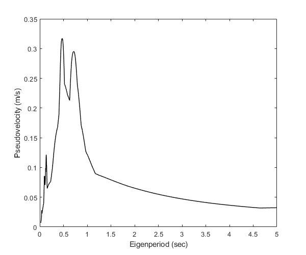
Pseudovelocity spectrum

figure()
plot(T,PSv,'k','LineWidth',1)
ylabel('Pseudovelocity (m/s)')
xlabel('Eigenperiod (sec)')
drawnow;
pause(0.1)

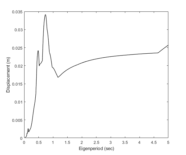
Displacement spectrum

figure()
plot(T,Sd,'k','LineWidth',1)
ylabel('Displacement (m)')
xlabel('Eigenperiod (sec)')
drawnow;
pause(0.1)

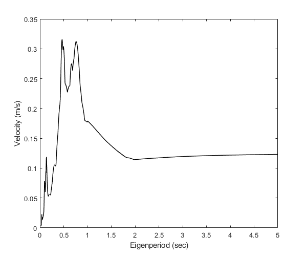
Velocity spectrum

figure()
plot(T,Sv,'k','LineWidth',1)
ylabel('Velocity (m/s)')
xlabel('Eigenperiod (sec)')
drawnow;
pause(0.1)

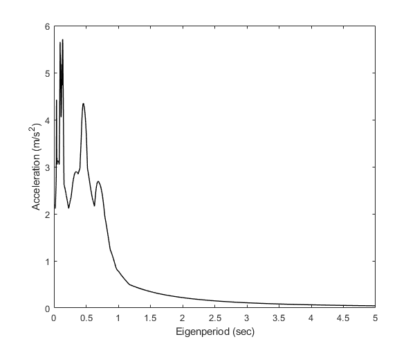
Acceleration spectrum

figure()
plot(T,Sa,'k','LineWidth',1)
ylabel('Acceleration (m/s^2)')
xlabel('Eigenperiod (sec)')
drawnow;
pause(0.1)

Equivalent relative input energy velocity

figure()
plot(T,Siev,'k','LineWidth',1)
ylabel('Equivalent relative input energy velocity (m/s)')
xlabel('Eigenperiod (sec)')
drawnow;
pause(0.1)

Copyright

Copyright (c) 2018-2023 by George Papazafeiropoulos

Published with MATLAB® R2022b