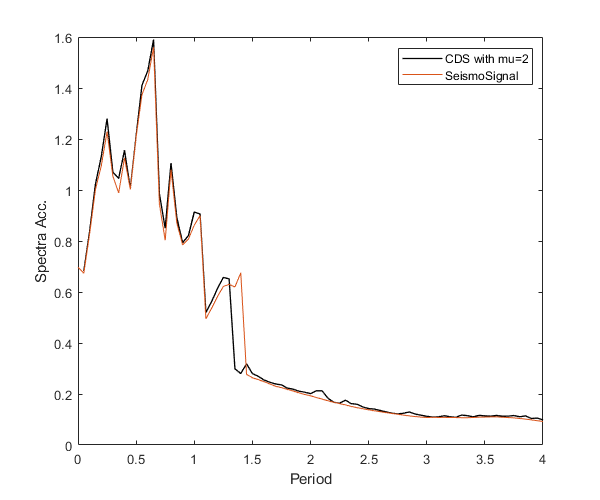
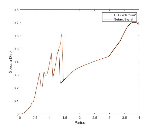
example Comparison of constant ductility response spectra of RSN1044 for mu=2

Input
Results from OpenSeismoMatlab
Results from SeismoSignal
Output
Copyright

Input

Earthquake motions

GMFileLoc = 'input\';

A text file containing the lists of GM names

RecordList = ['input\Record_List.txt'];

Read E.Q. records name from the specifid list

fid = fopen (RecordList,'r');
records = textscan(fid, '%s'); % length = num of records*1, cell
fclose (fid);

Read E.Q. records name from the specifid list Return variables include record names, dt, num of points, PGA, Acc TH, Spectral Acc The accelration-related variables (PGA, Sa, Acc TH) are in unit of g; disp-related in m If you do not specify scaling factors at this step, the default value = 1 for each GM

[RecordName_all, dt, numPoint_all, PGA_all, xgtt] =...
    fn_ParseAT2File2(GMFileLoc, records);

Set the eigenperiod range for which the response spectra will be calculated.

Tspectra=(0.05:0.05:4)';

Set critical damping ratio of the response spectra to be calculated.

ksi=0.02;

Results from OpenSeismoMatlab

Set the target ductility

mu=2; % mu=1 equivalent to a linear SDoF

Extract constant ductility response spectra

sw='cdrs';

Calculation CDRS{i}=[S.Period,S.CDSd,S.CDSv,S.CDPSa,S.fyK,S.muK,S.iterK];

S1=OpenSeismoMatlab(dt,xgtt{1},sw,Tspectra,ksi,mu);

Results from SeismoSignal

fileID = fopen('input/RSN1044_Damping2.txt');
for idx = 1:5
    fgetl(fileID);
end
C = textscan(fileID,repmat('%f',1,15));
fclose(fileID);

Output

Plot spectral acceleration response spectra

figure()
plot(S1.Period,S1.CDSa/9.8,'k','LineWidth',1);
hold on
%plot(S2.Period,S2.Sa,'r','LineWidth',1);
plot(C{1},C{3})
legend('CDS with mu=2','SeismoSignal');
xlabel('Period');
ylabel('Spectra Acc.')
hold off
drawnow;
pause(0.1)

Plot spectral velocity response spectra

figure()
plot(S1.Period,S1.CDSv,'k','LineWidth',1);
hold on
%plot(S2.Period,S2.Sa,'r','LineWidth',1);
plot(C{1},C{7}/100)
legend('CDS with mu=2','SeismoSignal');
xlabel('Period');
ylabel('Spectra Vel.')
hold off
drawnow;
pause(0.1)

Plot spectral displacement response spectra

figure()
plot(S1.Period,S1.CDSd,'k','LineWidth',1);
hold on
%plot(S2.Period,S2.Sa,'r','LineWidth',1);
plot(C{1},C{11}/100)
legend('CDS with mu=2','SeismoSignal');
xlabel('Period');
ylabel('Spectra Disp.')
hold off
drawnow;
pause(0.1)

Plot the achieved ductility for each eigenperiod. It should be equal or close to the target ductility mu=2

figure()
plot(S1.Period,S1.muK,'k','LineWidth',1);
xlabel('Period');
ylabel('Real mu values after iterations')
drawnow;
pause(0.1)

Copyright