example General demonstration of the OpenSeismoMatlab capabilities

This is to demonstrate the capabilities of OpenSeismoMatlab and also to verify that OpenSeismoMatlab works properly for all of its possible options and types of application, and yields meaningful results. All capabilities of OpenSeismoMatlab are tested in this example

Contents

Load earthquake data

Earthquake acceleration time history of the El Centro earthquake will be used (El Centro, 1940, El Centro Terminal Substation Building)

fid=fopen('elcentro_NS_trunc.dat','r');
text=textscan(fid,'%f %f');
fclose(fid);
t=text{1,1};
dt=t(2)-t(1);
xgtt=text{1,2};

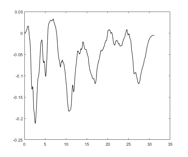
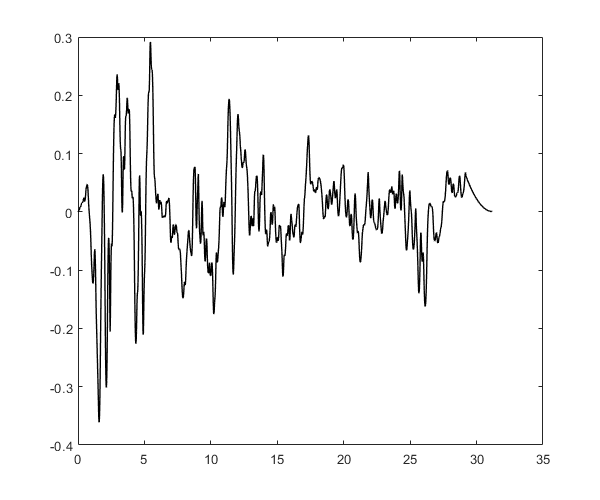
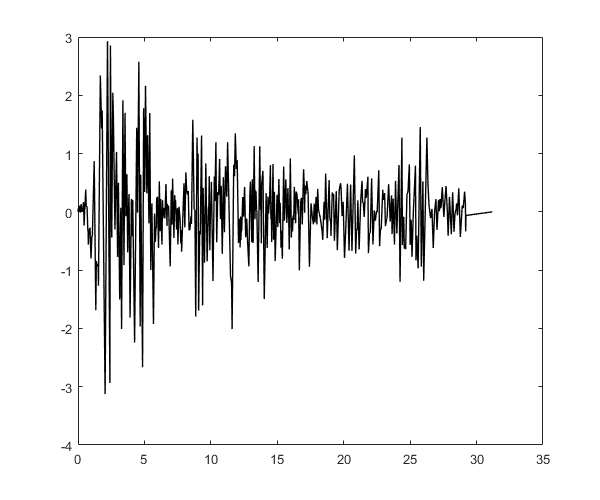
Time histories without baseline correction

sw='timehist';
baselineSw=false;
S1=OpenSeismoMatlab(dt,xgtt,sw,baselineSw);

figure()
plot(S1.time,S1.disp,'k','LineWidth',1)
drawnow;
pause(0.1)

figure()
plot(S1.time,S1.vel,'k','LineWidth',1)
drawnow;
pause(0.1)

figure()
plot(S1.time,S1.acc,'k','LineWidth',1)
drawnow;
pause(0.1)

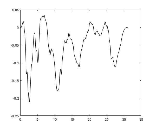
Time histories with baseline correction

sw='timehist';
baselineSw=true;
S2=OpenSeismoMatlab(dt,xgtt,sw,baselineSw);

figure()
plot(S2.time,S2.disp,'k','LineWidth',1)
drawnow;
pause(0.1)

figure()
plot(S2.time,S2.vel,'k','LineWidth',1)
drawnow;
pause(0.1)

figure()
plot(S2.time,S2.acc,'k','LineWidth',1)
drawnow;
pause(0.1)

Resample acceleration time history from 0.02 sec to 0.01 sec.

sw='sincresample';
dti=0.01;
S3=OpenSeismoMatlab(dt,xgtt,sw,dti);

figure()
plot(S3.time,S3.acc,'k','LineWidth',1)
drawnow;
pause(0.1)

PGA

sw='pga';
S4=OpenSeismoMatlab(dt,xgtt,sw);

S4.PGA

ans =

                 3.1276242

PGV

sw='pgv';
S5=OpenSeismoMatlab(dt,xgtt,sw);

S5.PGV

ans =

               0.360920691

PGD

sw='pgd';
S6=OpenSeismoMatlab(dt,xgtt,sw);

S6.PGD

ans =

         0.211893410160001

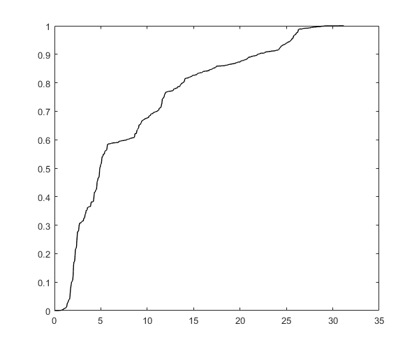
Total cumulative energy, Arias intensity and significant duration

sw='arias';
S7=OpenSeismoMatlab(dt,xgtt,sw);

S7.Ecum

ans =

           11.251388628142

figure()
plot(S7.time,S7.EcumTH,'k','LineWidth',1)
drawnow;
pause(0.1)

S7.t_5_95

ans =

                      1.68                      25.5

S7.Td_5_95

ans =

                     23.84

S7.t_5_75

ans =

                      1.68                      11.8

S7.Td_5_75

ans =

                     10.14

S7.arias

ans =

          1.80159428424335

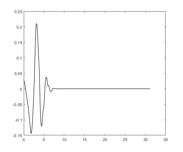
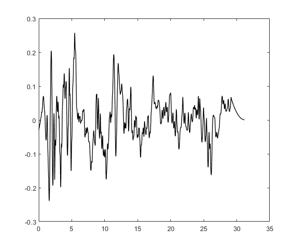
Pulse decomposition

xgt=S1.vel;
sw='pulsedecomp';
S8=OpenSeismoMatlab(dt,xgt,sw);

figure()
plot(S8.time,S8.pulseTH,'k','LineWidth',1)
drawnow;
pause(0.1)

figure()
plot(S8.time,S8.resTH,'k','LineWidth',1)
drawnow;
pause(0.1)

S8.Tp

ans =

                     3.304

S8.wavScale

ans =

   118

S8.wavCoefs

ans =

          1.71247132221248

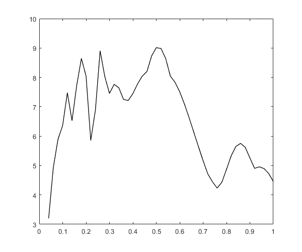
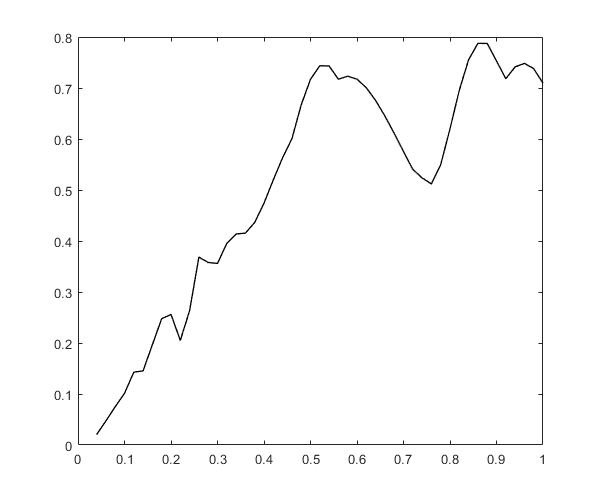
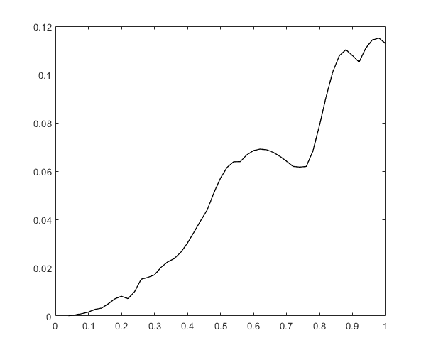
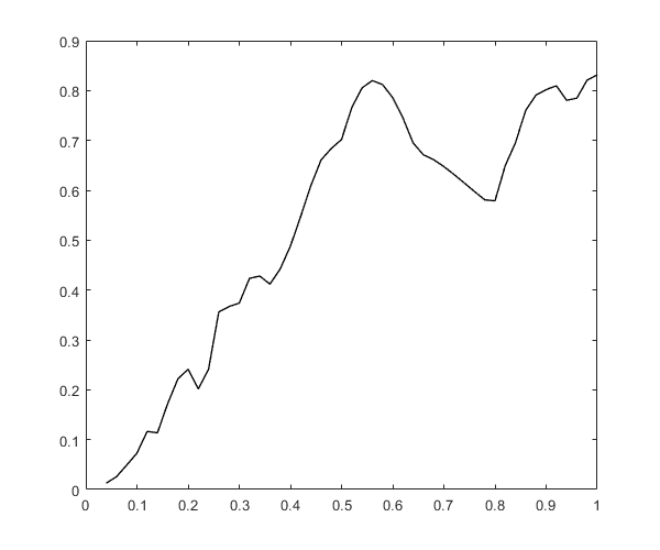
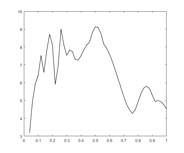
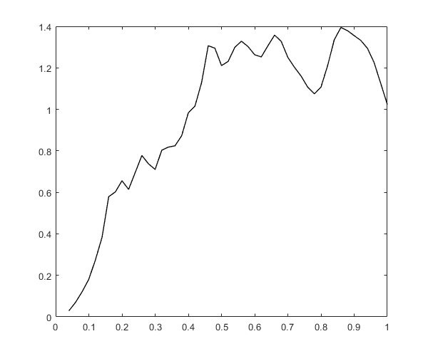
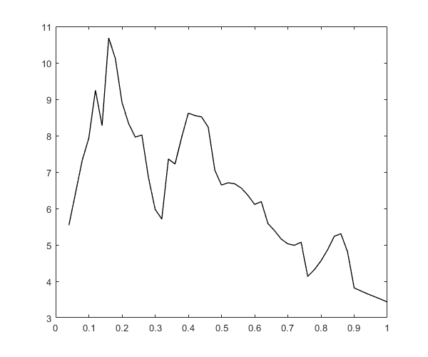
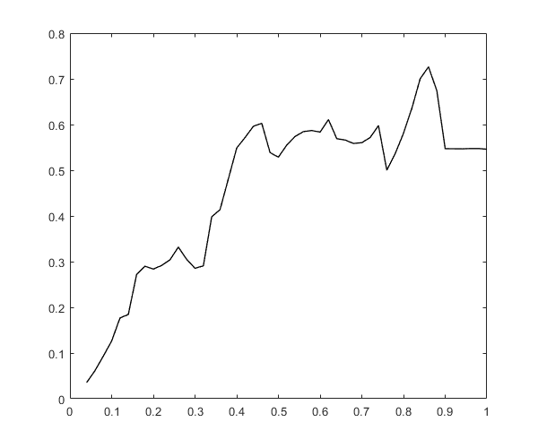
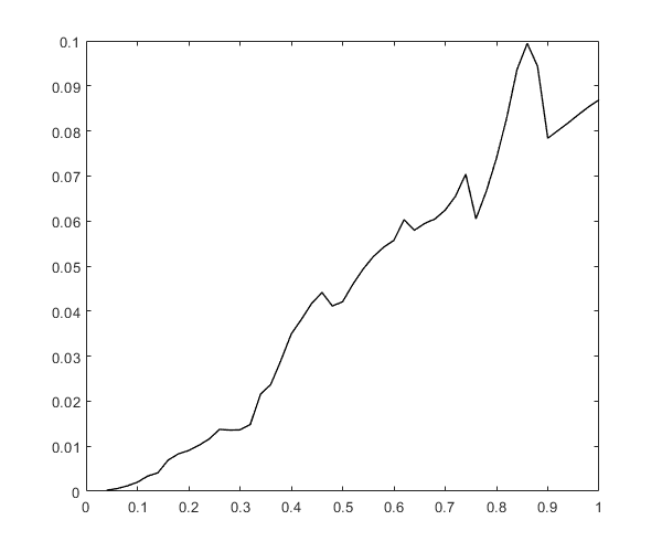
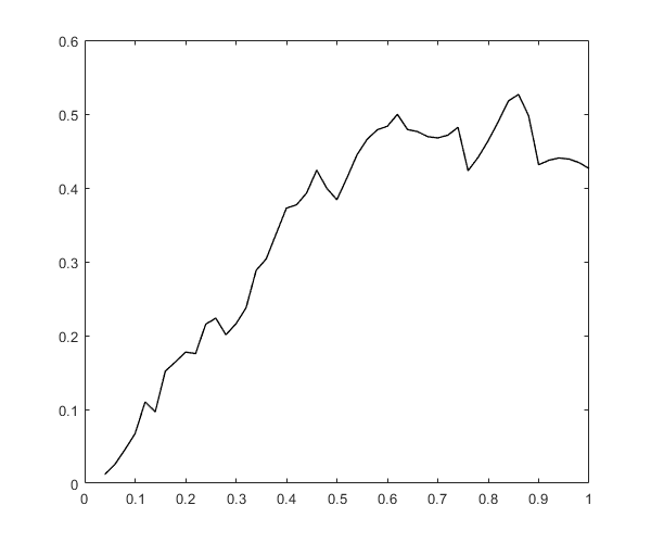
Linear elastic response spectra and pseudospectra

sw='elrs';
ksi=0.05;
T=0.04:0.02:1;
S9=OpenSeismoMatlab(dt,xgtt,sw,T,ksi);

figure()
plot(S9.Period,S9.PSa,'k','LineWidth',1)
drawnow;
pause(0.1)

figure()
plot(S9.Period,S9.PSv,'k','LineWidth',1)
drawnow;
pause(0.1)

figure()
plot(S9.Period,S9.Sd,'k','LineWidth',1)
drawnow;
pause(0.1)

figure()
plot(S9.Period,S9.Sv,'k','LineWidth',1)
drawnow;
pause(0.1)

figure()
plot(S9.Period,S9.Sa,'k','LineWidth',1)
drawnow;
pause(0.1)

figure()
plot(S9.Period,S9.Siev,'k','LineWidth',1)
drawnow;
pause(0.1)

S9.PredPSa

ans =

          9.01181525615902

S9.PredPeriod

ans =

                       0.5

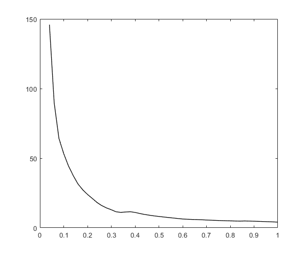
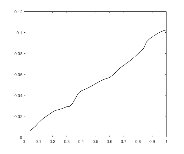
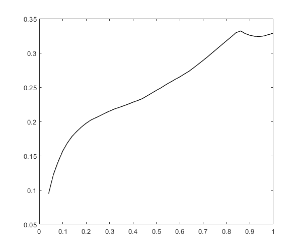
Rigid plastic sliding displacement response spectra

sw='rpsrs';
S10=OpenSeismoMatlab(dt,xgtt,sw);

figure()
plot(S10.CF,S10.RPSSd,'k','LineWidth',1)
drawnow;
pause(0.1)

figure()
plot(S10.CF,S10.RPSSv,'k','LineWidth',1)
drawnow;
pause(0.1)

figure()
plot(S10.CF,S10.RPSSa,'k','LineWidth',1)
drawnow;
pause(0.1)

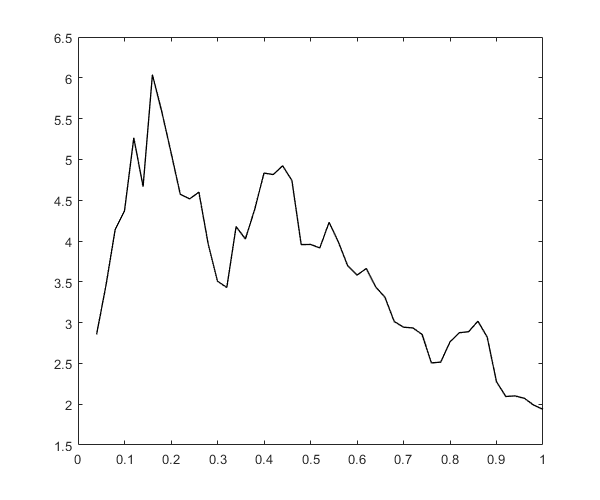
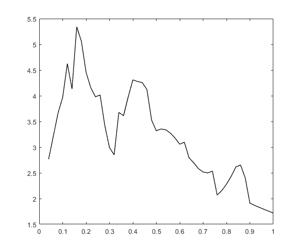
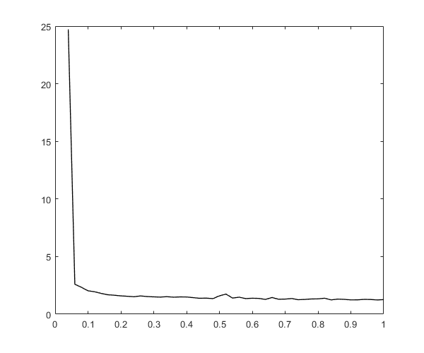
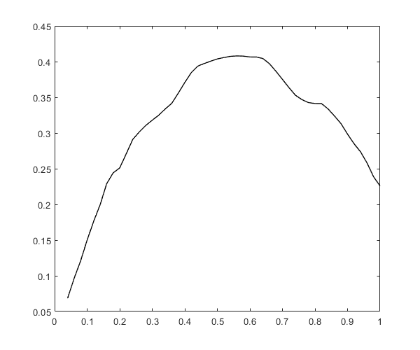
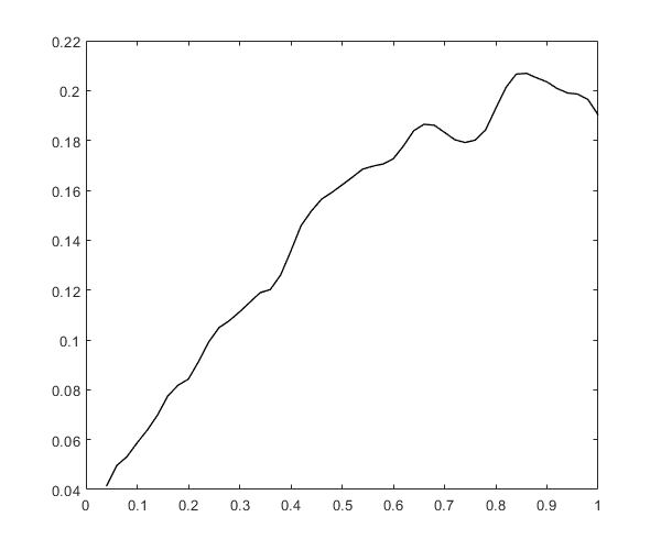
Constant ductility response spectra and pseudospectra

sw='cdrs';
ksi=0.05;
T=0.04:0.02:1;
mu=2;
S11=OpenSeismoMatlab(dt,xgtt,sw,T,ksi,mu);

figure()
plot(S11.Period,S11.CDPSa,'k','LineWidth',1)
drawnow;
pause(0.1)

figure()
plot(S11.Period,S11.CDPSv,'k','LineWidth',1)
drawnow;
pause(0.1)

figure()
plot(S11.Period,S11.CDSd,'k','LineWidth',1)
drawnow;
pause(0.1)

figure()
plot(S11.Period,S11.CDSv,'k','LineWidth',1)
drawnow;
pause(0.1)

figure()
plot(S11.Period,S11.CDSa,'k','LineWidth',1)
drawnow;
pause(0.1)

figure()
plot(S11.Period,S11.fyK,'k','LineWidth',1)
drawnow;
pause(0.1)

figure()
plot(S11.Period,S11.muK,'k','LineWidth',1)
drawnow;
pause(0.1)

figure()
plot(S11.Period,S11.iterK,'k','LineWidth',1)
drawnow;
pause(0.1)

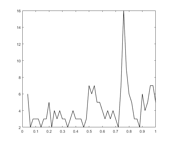
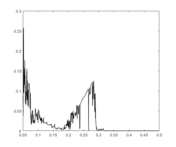
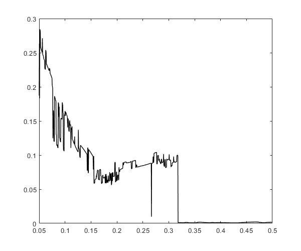
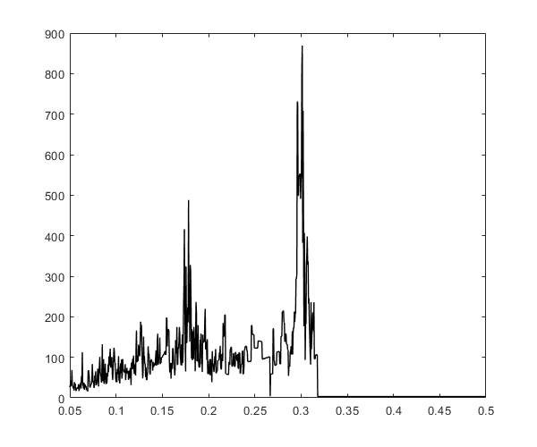
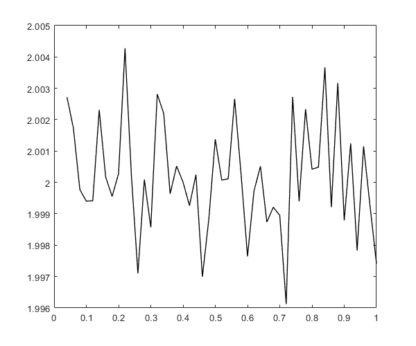
Constant strength response spectra

sw='csrs';
ksi=0.05;
T=0.04:0.02:1;
fyR=0.1;
S12=OpenSeismoMatlab(dt,xgtt,sw,T,ksi,fyR);

figure()
plot(S12.Period,S12.CSSmu,'k','LineWidth',1)
drawnow;
pause(0.1)

figure()
plot(S12.Period,S12.CSSd,'k','LineWidth',1)
drawnow;
pause(0.1)

figure()
plot(S12.Period,S12.CSSv,'k','LineWidth',1)
drawnow;
pause(0.1)

figure()
plot(S12.Period,S12.CSSa,'k','LineWidth',1)
drawnow;
pause(0.1)

figure()
plot(S12.Period,S12.CSSey,'k','LineWidth',1)
drawnow;
pause(0.1)

figure()
plot(S12.Period,S12.CSSed,'k','LineWidth',1)
drawnow;
pause(0.1)

Fourier amplitude spectrum and mean period

sw='fas';
S13=OpenSeismoMatlab(dt,xgtt,sw);

figure()
plot(S13.freq,S13.FAS,'k','LineWidth',1)
drawnow;
pause(0.1)

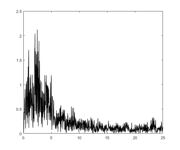
S13.Tm

ans =

         0.514862185011529

S13.Fm

ans =

          3.55564226051675

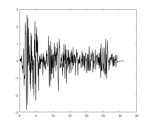
High pass Butterworth filter

sw='butterworthhigh';
bOrder=4;
flc=0.1;
S14=OpenSeismoMatlab(dt,xgtt,sw,bOrder,flc);

figure()
plot(S14.time,S14.acc,'k','LineWidth',1)
drawnow;
pause(0.1)

Low pass Butterworth filter

sw='butterworthlow';
bOrder=4;
fhc=10;
S15=OpenSeismoMatlab(dt,xgtt,sw,bOrder,fhc);

figure()
plot(S15.time,S15.acc,'k','LineWidth',1)
drawnow;
pause(0.1)

Incremental dynamic analysis

sw='ida';
S16=OpenSeismoMatlab(dt,xgtt,sw);

figure()
plot(S16.DM,S16.IM,'k','LineWidth',1)
drawnow;
pause(0.1)

Effective peak ground acceleration

sw='epga';
S17=OpenSeismoMatlab(dt,xgtt,sw);

S17.EPGA

ans =

          3.09546779631066

Spectral intensity according to Housner (1952)

sw='sih1952';
S18=OpenSeismoMatlab(dt,xgtt,sw);

S18.SI

ans =

          1.24373311662318

Spectral intensity according to Nau & Hall (1984)

sw='sinh1984';
S19=OpenSeismoMatlab(dt,xgtt,sw);

S19.SI

ans =

         0.530561283239986

Copyright

Copyright (c) 2018-2023 by George Papazafeiropoulos

Published with MATLAB® R2022b