verification Constant ductility response spectrum

Contents

Reference

Chopra, A. K. (2020). Dynamics of structures, Theory and Applications to Earthquake Engineering, 5th edition. Prenctice Hall.

Description

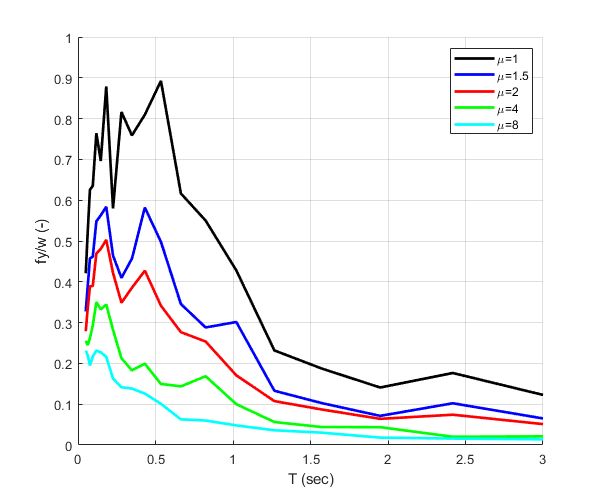
The constant-ductility response spectra of Figure 7.5.2 of the above reference are verified. Elastic-perfectly plastic systems are considered. Damping is equal to 5% of its critical value. Target ductility factors equal to 1,1.5,2,4 and 8 are considered.

Load earthquake data

Earthquake acceleration time history of the El Centro earthquake will be used (El Centro, 1940, El Centro Terminal Substation Building)

fid=fopen('elcentro_NS_trunc.dat','r');
text=textscan(fid,'%f %f');
fclose(fid);
t=text{1,1};
dt=t(2)-t(1);
xgtt=text{1,2};

Calculate constant ductility response spectra of earthquake motion

Switch

sw='cdrs';

Eigenperiods

T=logspace(log10(0.05),log10(3),20);

Critical damping ratio

ksi=0.05;

Ductilities

mu1=1;
mu2=1.5;
mu3=2;
mu4=4;
mu5=8;

Post-yield stiffness factor

pysf=0.001;

Apply OpenSeismoMatlab once for each target ductility value

S1=OpenSeismoMatlab(dt,xgtt,sw,T,ksi,mu1,pysf);
S2=OpenSeismoMatlab(dt,xgtt,sw,T,ksi,mu2,pysf);
S3=OpenSeismoMatlab(dt,xgtt,sw,T,ksi,mu3,pysf);
S4=OpenSeismoMatlab(dt,xgtt,sw,T,ksi,mu4,pysf);
S5=OpenSeismoMatlab(dt,xgtt,sw,T,ksi,mu5,pysf);

Plot the constant ductility response spectra

Initialize figure

figure()
hold on
% Plot the constant ductility response spectra
plot(S1.Period,S1.fyK/9.81, 'k-', 'LineWidth', 2)
plot(S2.Period,S2.fyK/9.81, 'b-', 'LineWidth', 2)
plot(S3.Period,S3.fyK/9.81, 'r-', 'LineWidth', 2)
plot(S4.Period,S4.fyK/9.81, 'g-', 'LineWidth', 2)
plot(S5.Period,S5.fyK/9.81, 'c-', 'LineWidth', 2)
hold off
% Finalize figure
grid on
xlabel('T (sec)')
ylabel('fy/w (-)')
legend({'\mu=1','\mu=1.5','\mu=2','\mu=4','\mu=8'})
xlim([0,3])
ylim([0,1])
drawnow;
pause(0.1)

Copyright

Copyright (c) 2018-2023 by George Papazafeiropoulos

Published with MATLAB® R2022b