verification Incremental dynamic analysis for ductility response

Contents

Reference

De Luca, F., Vamvatsikos, D., & Iervolino, I. (2011, May). Near-optimal bilinear fit of capacity curves for equivalent SDOF analysis. In Proceedings of the COMPDYN2011 Conference on Computational Methods in Structural Dynamics and Earthquake Engineering, Corfu, Greece.

Description

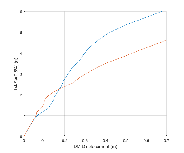
Figure 1(b) of the above reference presents the median IDA curves of SDOF systems with T=0.5sec. The actual capacity curve of the SDOF oscillator shown in FIgure 1(a) of the same reference (green line), has been fitted with an elastoplastic bilinear fit according to FEMA-440 (blue line). This fitting introduces an error (bias) which appears as the blue area in Figure 1(b), which is generally conservative. In this example two arbitrary acceleration time histories are selected, then the corresponding displacement response IDA curves are plotted, based on a SDOF system with suitably selected properties, based on Figure 1(a). It is shown that both curves approximately fall into the bias (blue area) of Figure 1(b) of the above reference.

Earthquake motions

Load data from two earthquakes

GM={'Imperial Valley'; % Imperial valley 1979
    'Cape Mendocino'};
n=size(GM,1);
dt=cell(n,1);
xgtt=cell(n,1);
for i=1:n
    fid=fopen([GM{i},'.dat'],'r');
    text=textscan(fid,'%f %f');
    fclose(fid);
    t=text{1,1};
    dt{i}=t(2)-t(1);
    xgtt{i}=text{1,2};
end

Setup parameters for IDA analysis

Switch

sw='ida';

Eigenperiod

T=0.5;

Scaling factors

lambdaF=logspace(log10(0.01),log10(30),100);

Type of IDA analysis

IM_DM='Sa_disp';

Yield displacement

uy=0.042;

Initial stiffness

k_hi=1000/uy;

Mass

m=k_hi/(2*pi/T)^2;

Post yield stiffness factor

pysf=0.01;

Fraction of critical viscous damping

ksi=0.05;

Algorithm to be used for the time integration

AlgID='U0-V0-Opt';

Set initial displacement

u0=0;

Set initial velocity

ut0=0;

Minimum absolute value of the eigenvalues of the amplification matrix

rinf=1;

Maximum tolerance for convergence

maxtol=0.01;

Maximum number of iterations per increment

jmax=200;

Infinitesimal variation of acceleration

dak=eps;

Construct and plot the IDA curves in a loop

Initialize figure

figure()
hold on
% Plot the IDA curves of Figure 1(b) of the above reference
for i=1:n
    S1=OpenSeismoMatlab(dt{i},xgtt{i},sw,T,lambdaF,IM_DM,m,uy,pysf,ksi,AlgID,...
        u0,ut0,rinf,maxtol,jmax,dak);
    plot(S1.DM,S1.IM/9.81)
end
% Finalize figure
grid on
xlabel('DM-Displacement (m)')
ylabel('IM-Sa(T,5%) (g)')
xlim([0,0.7])
ylim([0,6])
drawnow;
pause(0.1)

Copyright

Copyright (c) 2018-2023 by George Papazafeiropoulos

Published with MATLAB® R2022b