verification of seismic input energy of linear SDOF oscillator

Compare the output of LIDA.m and NLIDABLKIN.m for a linear SDOF oscillator in terms of seismic input energy per unit mass.

Contents

Reference

None

Description

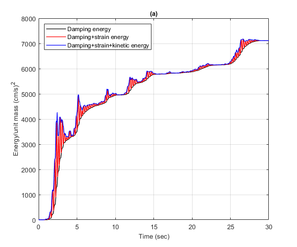
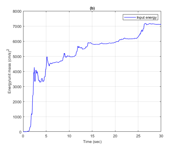
Calculate the time histories of the various energies that are absorbed by a linear elastic SDOF oscillator using the linear function LIDA.m and the nonlinear function NLIDABLKIN.m to which an infinite yield limit has been assigned. The time history of the seismic input energy per unit mass obtained by the LIDA.m function (Figure b) is compared to the sum of the strain, damping and kinetic energies per unit mass obtained by the NLIDABLKIN.m function (Figure a). The linear SDOF system has Tn=0.5 sec and ksi=5%.

Load earthquake data

Earthquake acceleration time history of the El Centro earthquake will be used (El Centro, 1940, El Centro Terminal Substation Building)

fid=fopen('elcentro_NS_trunc.dat','r');
text=textscan(fid,'%f %f');
fclose(fid);
t=text{1,1};
dt=t(2)-t(1);
xgtt=text{1,2};

Setup parameters for NLIDABLKIN function for linear SDOF

Mass

m=1;

Eigenperiod

Tn=0.5;

Calculate the small-strain stiffness matrix

omega=2*pi/Tn;
k_hi=m*omega^2;

Assign linear elastic properties

k_lo=k_hi;
uy1=1e10;

Critical damping ratio

ksi=0.05;

Initial displacement

u0=0;

Initial velocity

ut0=0;

Algorithm to be used for the time integration

AlgID='U0-V0-Opt';

Minimum absolute value of the eigenvalues of the amplification matrix

rinf=1;

Maximum tolerance of convergence for time integration algorithm

maxtol=0.01;

Maximum number of iterations per integration time step

jmax=200;

Infinitesimal acceleration

dak=eps;

Calculate dynamic response of linear SDOF using NLIDABLKIN.m

Apply NLIDABLKIN

[u,ut,utt,Fs,Ey,Es,Ed,jiter] = NLIDABLKIN(dt,xgtt,m,k_hi,k_lo,uy1,...
    ksi,AlgID,u0,ut0,rinf,maxtol,jmax,dak);

Calculate the kinetic energy of SDOF

Ek=1/2*m*ut.^2;

Plot the energy time histories of the linear SDOF

Plot the damping energy, damping plus strain energy, damping plus strain plus kinetic energy of the linearly elastic SDOF system. Convert from m to cm

figure()
plot(t',cumsum(Ed)*1e4,'k','LineWidth',1)
hold on
plot(t',cumsum(Ed)*1e4+Es*1e4,'r','LineWidth',1)
plot(t',cumsum(Ed)*1e4+Es*1e4+Ek*1e4,'b','LineWidth',1)
hold off
xlim([0,30])
ylim([0,8000])
xlabel('Time (sec)','FontSize',10);
ylabel('Energy/unit mass (cm/s)^2','FontSize',10);
title('(a)','FontSize',10)
grid on
legend({'Damping energy','Damping+strain energy',...
    'Damping+strain+kinetic energy'},'location','northwest')
drawnow;
pause(0.1)

Calculate dynamic response of the linear SDOF using LIDA.m

Apply the LIDA.m function for the linear SDOF

[u,ut,utt,Ei] = LIDA(dt,xgtt,omega,ksi,u0,ut0,AlgID,rinf);

Plot the energy time history of the nonlinear SDOF

Plot the damping energy, the hysteretic energy and strain energy of the nonlinear SDOF system. Convert from m to cm.

figure();
plot(t,cumsum(Ei)*1e4,'b','LineWidth',1)
xlim([0,30])
ylim([0,8000])
xlabel('Time (sec)','FontSize',10);
ylabel('Energy/unit mass (cm/s)^2','FontSize',10);
title('(b)','FontSize',10)
grid on
legend('Input energy')
drawnow;
pause(0.1)

Copyright

Copyright (c) 2018-2023 by George Papazafeiropoulos

Published with MATLAB® R2022b