verification Energy time history of SDOF oscillator

Calculate the time history of the strain energy and the energy dissipated by viscous damping and yielding of a linear and a nonlinear SDOF oscillator

Reference
Description
Load earthquake data
Setup parameters for NLIDABLKIN function for linear SDOF
Calculate dynamic response of the linear SDOF
Plot the energy time history of the linear SDOF
Setup parameters for NLIDABLKIN function for nonlinear SDOF
Calculate dynamic response of the nonlinear SDOF
Plot the energy time history of the nonlinear SDOF
Copyright

Reference

Chopra, A. K. (2020). Dynamics of structures, Theory and Applications to Earthquake Engineering, 5th edition. Prenctice Hall.

Description

Figure 7.9.1 of the above reference is reproduced in this example, for both the linear elastic and the elastoplastic SDOF systems. The linear system has Tn=0.5 sec and ksi=5%, whereas the elastoplastic system has Tn=0.5 sec, ksi=5% and fybar=0.25.

Load earthquake data

Earthquake acceleration time history of the El Centro earthquake will be used (El Centro, 1940, El Centro Terminal Substation Building)

fid=fopen('elcentro_NS_trunc.dat','r');
text=textscan(fid,'%f %f');
fclose(fid);
t=text{1,1};
dt=t(2)-t(1);
xgtt=text{1,2};

Setup parameters for NLIDABLKIN function for linear SDOF

Mass

m=1;

Eigenperiod

Tn=0.5;

Calculate the small-strain stiffness matrix

omega=2*pi/Tn;
k_hi=m*omega^2;

Assign linear elastic properties

k_lo=k_hi;
uy1=1e10;

Critical damping ratio

ksi=0.05;

Initial displacement

u0=0;

Initial velocity

ut0=0;

Algorithm to be used for the time integration

AlgID='U0-V0-Opt';

Minimum absolute value of the eigenvalues of the amplification matrix

rinf=1;

Maximum tolerance of convergence for time integration algorithm

maxtol=0.01;

Maximum number of iterations per integration time step

jmax=200;

Infinitesimal acceleration

dak=eps;

Calculate dynamic response of the linear SDOF

Apply NLIDABLKIN

[u,ut,utt,Fs,Ey,Es,Ed,jiter] = NLIDABLKIN(dt,xgtt,m,k_hi,k_lo,uy1,...
    ksi,AlgID,u0,ut0,rinf,maxtol,jmax,dak);

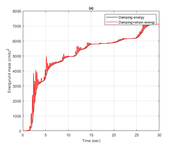
Plot the energy time history of the linear SDOF

Plot the damping energy and strain energy of the linearly elastic SDOF system. Convert from m to cm

figure()
plot(t',cumsum(Ed)*1e4,'k','LineWidth',1)
hold on
plot(t',cumsum(Ed)*1e4+Es*1e4,'r','LineWidth',1)
hold off
xlim([0,30])
ylim([0,8000])
xlabel('Time (sec)','FontSize',10);
ylabel('Energy/unit mass (cm/s)^2','FontSize',10);
title('(a)','FontSize',10)
grid on
legend('Damping energy','Damping+strain energy')
drawnow;
pause(0.1)

Setup parameters for NLIDABLKIN function for nonlinear SDOF

The properties of the nonlinear SDOF system are identical to those of the linear SDOF system, except for the yield displacement and the post-yield stiffness.

Post yield stiffness

k_lo=0.01*k_hi;

normalized yield strength

fybar=0.25;

Yield displacement for nonlinear response

uy2=fybar*max(abs(u));

Calculate dynamic response of the nonlinear SDOF