verification Pulse Decomposition of OpenSeismoMatlab

Contents

Reference

Shahi, S. K., & Baker, J. W. (2014). An efficient algorithm to identify strong‐velocity pulses in multicomponent ground motions. Bulletin of the Seismological Society of America, 104(5), 2456-2466.

Description

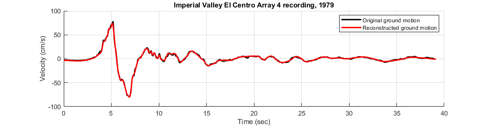
The velocity pulses of a strong motion velocity time history are extracted according to Figure 3 of the above reference, and the extracted pulses are summed to give the reconstructed ground motion. There is significant agreement between the original and the reconstructed ground motions. The velocity time history of the 1979 Imperial Valley El Centro Array 4 recording is considered. The Daubechies wavelet of order 4 is used as the mother wavelet.

Earthquake motion

Load earthquake data of 1979 Imperial Valley El Centro Array 4 recording

eqmotion={'ImperialValleyElCentroArray4.txt'};
data=load(eqmotion{1});
t=data(:,1);
dt=t(2)-t(1);
xgt=data(:,2);

Perform pulse decomposition of earthquake motion

Switch

sw='pulsedecomp';

Wavelet family of Daubechies wavelet of order 4

wname = 'db4';

Apply OpenSeismoMatlab for extracting the first 30 largest pulses from the initial motion

S1=OpenSeismoMatlab(dt,xgt,sw,wname);
Sout{1}=S1;
for i=2:30
    S1=OpenSeismoMatlab(dt,S1.resTH,sw,wname);
    Sout{i}=S1;
end

Sum the 30 largest pulses extracted from the input motion

sum30=zeros(size(S1.pulseTH));
for i=1:30
    sum30=sum30+Sout{i}.pulseTH;
end

Plot the velocity time histories (original and reconstructed)

Initialize figure

figure('Position',[7.4,508.2,1517.6,253.8],...
    'InnerPosition',[7.4,508.2,1517.6,253.8],...
    'OuterPosition',[0.2,501,1000,343.2])
hold on
% Plot the velocity time history of the original ground motion
plot(t,xgt, 'Color', [0 0 0], 'LineWidth', 2)
% Plot the velocity time history of the reconstructed ground motion
plot(t,sum30, 'Color', [1 0 0], 'LineWidth', 2)
% Finalize figure
hold off
grid on
title('Imperial Valley El Centro Array 4 recording, 1979')
ylim([-100,100])
xlim([0,40])
xlabel('Time (sec)')
ylabel('Velocity (cm/s)')
legend({'Original ground motion','Reconstructed ground motion'})
drawnow;
pause(0.1)

Plot the 30 velocity pulses in a single plot

Verify with the middle plot of Figure 3 Initialize figure

figure('Position',[5	50.6	1524.8	731.2],...
    'InnerPosition',[5	50.6	1524.8	731.2],...
    'OuterPosition',[-2.20	43.4	1000	820.8])
hold on
offSet=0;
for i=1:30
    offSet=offSet+abs(min(Sout{i}.pulseTH));
    plot(t,offSet+Sout{i}.pulseTH, 'Color', [0.7 0.7 0.7], 'LineWidth', 2)
    offSet=offSet+max(Sout{i}.pulseTH);
end
% Finalize figure
hold off
grid on
title('Imperial Valley El Centro Array 4 recording, 1979')
ylim([0,450])
set(gca, 'YDir','reverse')
xlim([0,40])
xlabel('Time (sec)')
ylabel('Velocity (cm/s)')
drawnow;
pause(0.1)

Copyright

Copyright (c) 2018-2023 by George Papazafeiropoulos

Published with MATLAB® R2022b