verification Rigid plastic sliding response spectrum

Contents

Reference

Garini, E., & Gazetas, G. (2016). Rocking and Sliding Potential of the 2014 Cephalonia, Greece Earthquakes. In ICONHIC2016 1st international conference on natural hazards & infrastructure June, Chania, Greece.

Description

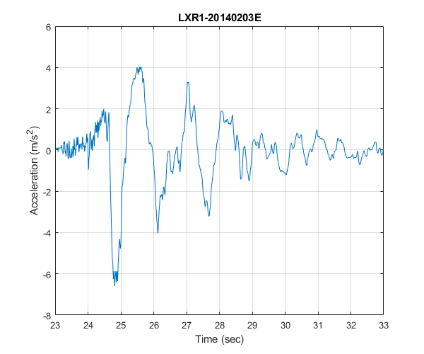
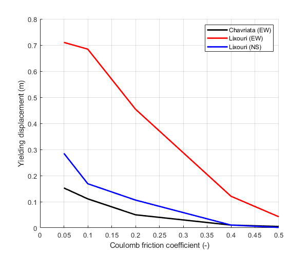
The rigid plastic sliding response spectra are extracted for various acceleration time histories of the 3 Feb 2014 13.34 EST Cephalonia earthquake. Three records are used: Chavriata (EW), Lixouri (EW) and Lixouri (NS). The oscillator is considered to be ideally rigid-plastic sliding on horizontal plane, as shown in Figure 4(a) of the above reference. The acceleration time histories that are used for the extraction of the spectra are plotted in this example and also shown in Figure 2 of the above reference [Chavriata (3 February) EW, Lixouri (3 February) EW, Lixouri (3 February) NS]. The rigid plastic sliding response spectra extracted in this example are compared to the corresponding spectra that appear in Figure 6 of the above reference.

Earthquake motions

Load earthquake data of Chavriata EW record

eqmotion={'CHV1-20140203E'};
data=load([eqmotion{1},'.txt']);
t1=data(:,1);
dt1=t1(2)-t1(1);
xgtt1=data(:,2)/100;
% Truncate the record
ind=t1>23 & t1<33;
xgtt1=xgtt1(ind);
t1=t1(ind);

Load earthquake data of Lixouri EW record

eqmotion={'LXR1-20140203E'};
data=load([eqmotion{1},'.txt']);
t2=data(:,1);
dt2=t2(2)-t2(1);
xgtt2=data(:,2)/100;
% Truncate the record
ind=t2>23 & t2<33;
xgtt2=xgtt2(ind);
t2=t2(ind);

Load earthquake data of Lixouri NS record

eqmotion={'LXR1-20140203N'};
data=load([eqmotion{1},'.txt']);
t3=data(:,1);
dt3=t3(2)-t3(1);
xgtt3=data(:,2)/100;
% Truncate the record
ind=t3>23 & t3<33;
xgtt3=xgtt3(ind);
t3=t3(ind);

Calculate rigid plastic sliding response spectrum of earthquake motion

Switch

sw='rpsrs';

Coulomb friction coefficients

CF=[0.05;0.1;0.2;0.4;0.5];

Apply OpenSeismoMatlab once for each record

S1=OpenSeismoMatlab(dt1,xgtt1,sw,CF);
S2=OpenSeismoMatlab(dt2,xgtt2,sw,CF);
S3=OpenSeismoMatlab(dt3,xgtt3,sw,CF);

Plot the acceleration time histories of the earthquake motions

Initialize figure

figure()
% Plot the acceleration time history
plot(t1,xgtt1)
% Finalize figure
grid on
title('CHV1-20140203E')
xlabel('Time (sec)')
ylabel('Acceleration (m/s^2)')
drawnow;
pause(0.1)

Initialize figure

figure()
% Plot the acceleration time history
plot(t2,xgtt2)
% Finalize figure
grid on
title('LXR1-20140203E')
xlabel('Time (sec)')
ylabel('Acceleration (m/s^2)')
drawnow;
pause(0.1)

Initialize figure

figure()
% Plot the acceleration time history
plot(t3,xgtt3)
% Finalize figure
grid on
title('LXR1-20140203N')
xlabel('Time (sec)')
ylabel('Acceleration (m/s^2)')
drawnow;
pause(0.1)

Plot the rigid plastic sliding response spectra

Initialize figure

figure()
hold on
% Plot the rigid plastic sliding response spectra
plot(S1.CF,S1.RPSSd, 'k-', 'LineWidth', 2)
plot(S2.CF,S2.RPSSd, 'r-', 'LineWidth', 2)
plot(S3.CF,S3.RPSSd, 'b-', 'LineWidth', 2)
hold off
% Finalize figure
grid on
xlabel('Coulomb friction coefficient (-)')
ylabel('Yielding displacement (m)')
legend({'Chavriata (EW)','Lixouri (EW)','Lixouri (NS)'})
xlim([0,0.5])
drawnow;
pause(0.1)

Copyright

Copyright (c) 2018-2023 by George Papazafeiropoulos

Published with MATLAB® R2022b