verification Rigid plastic sliding response spectrum

Contents

Reference

Paglietti, A., & Porcu, M. C. (2001). Rigid–plastic approximation to predict plastic motion under strong earthquakes. Earthquake engineering & structural dynamics, 30(1), 115-126.

Description

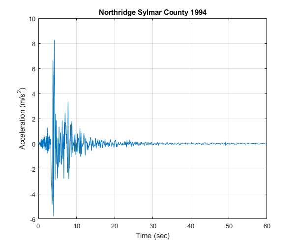
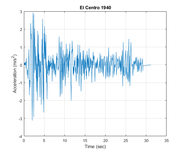
The rigid plastic sliding response spectra are extracted for two acceleration time histories: the Northridge (Sylmar County), Jan 1994 record and the El Centro, NS, May 1940 record, as presented in Table 1 of the above reference. The oscillator is considered to be ideally rigid-plastic sliding on horizontal plane. The acceleration time histories that are used for the extraction of the spectra are plotted in this example. The rigid plastic sliding response spectra extracted in this example are compared to the corresponding spectra that appear in Figure 6 of the above reference.

Earthquake motions

Load earthquake data of Northridge Sylmar County 1994 record

eqmotion={'Northridge_Sylmar_County'};
data=load([eqmotion{1},'.dat']);
t1=data(:,1);
dt1=t1(2)-t1(1);
xgtt1=data(:,2);

Load earthquake data of El Centro 1940 record

eqmotion={'elcentro_NS_trunc'};
data=load([eqmotion{1},'.dat']);
t2=data(:,1);
dt2=t2(2)-t2(1);
xgtt2=data(:,2);

Calculate rigid plastic sliding response spectrum of earthquake motion

Switch

sw='rpsrs';

Coulomb friction coefficients

CF1=[0.006;0.05;0.1;0.15;0.3;0.4;0.7;0.8];
CF2=[0.002;0.01;0.05;0.1;0.15;0.3;0.4];

Apply OpenSeismoMatlab once for each record

S1=OpenSeismoMatlab(dt1,xgtt1,sw,CF1);
S2=OpenSeismoMatlab(dt2,xgtt2,sw,CF2);

Plot the acceleration time histories of the earthquake motions

Initialize figure

figure()
% Plot the acceleration time history
plot(t1,xgtt1)
% Finalize figure
grid on
title('Northridge Sylmar County 1994')
xlabel('Time (sec)')
ylabel('Acceleration (m/s^2)')
drawnow;
pause(0.1)

Initialize figure

figure()
% Plot the acceleration time history
plot(t2,xgtt2)
% Finalize figure
grid on
title('El Centro 1940')
xlabel('Time (sec)')
ylabel('Acceleration (m/s^2)')
drawnow;
pause(0.1)

Plot the rigid plastic sliding response spectra

Initialize figure

figure()
% Plot the rigid plastic sliding response spectra
plot(S1.CF,S1.RPSSd, 'k-', 'LineWidth', 1)
% Finalize figure
grid on
xlabel('Coulomb friction coefficient (-)')
ylabel('Yielding displacement (m)')
title('Northridge Sylmar County 1994')
xlim([0,1])
drawnow;
pause(0.1)

Initialize figure

figure()
% Plot the rigid plastic sliding response spectra
plot(S2.CF,S2.RPSSd, 'k-', 'LineWidth', 1)
% Finalize figure
grid on
xlabel('Coulomb friction coefficient (-)')
ylabel('Yielding displacement (m)')
title('El Centro 1940')
xlim([0,0.5])
drawnow;
pause(0.1)

Copyright

Copyright (c) 2018-2023 by George Papazafeiropoulos

Published with MATLAB® R2022b