verification High pass Butterworth filter of OpenSeismoMatlab

Contents

Reference

Boore, D. M. (2005). On pads and filters: Processing strong-motion data. Bulletin of the Seismological Society of America, 95(2), 745-750.

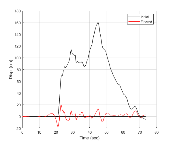
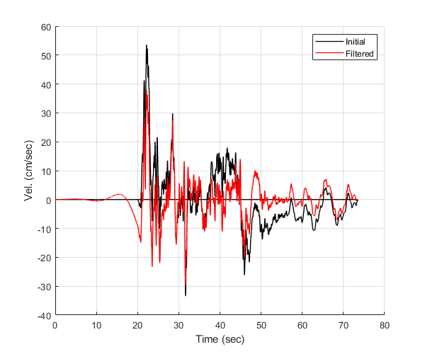
Description

Verify Figure 1 of the above reference, for the 1940 El Centro analog recording. The displacements and velocities from unfiltered and filtered accelerations are shown. Filtering is done by using two passes of a fourth-order high pass (i.e. frequencies lower than the cut-off frequency are attenuated) Butterworth filter with cut-off frequency as shown in Figure 1.

Earthquake motion

Load earthquake data

eqmotions={'Imperial_Valley_El_Centro_9_EW'};
data=load([eqmotions{1},'.dat']);
t=data(:,1);
dt=t(2)-t(1);
xgtt=data(:,2);

Apply high pass Butterworth filter

Switch

sw='butterworthhigh';

Order of Butterworth filter

bOrder=4;

Cut-off frequency

flc=0.1;

Apply OpenSeismoMatlab

S1=OpenSeismoMatlab(dt,xgtt,sw,bOrder,flc);

Filtered acceleration

cxgtt=S1.acc;

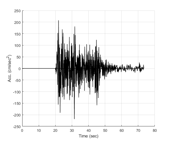
Plot the time history of the initial ground motion

Initialize figure

figure()
hold on
plot(t,zeros(size(t)),'k','LineWidth',1)
% Plot the acceleration time history of the initial ground motion
plot(t,xgtt,'k','LineWidth',1)
% Finalize figure
hold off
grid on
xlabel('Time (sec)')
ylabel('Acc. (cm/sec^2)')
drawnow;
pause(0.1)

Obtain displacement and velocity time histories

Switch

sw='timehist';

Do not use baseline correction

baselineSw=false;

Apply OpenSeismoMatlab to the initial ground motion

S2=OpenSeismoMatlab(dt,xgtt,sw,baselineSw);

Apply OpenSeismoMatlab to the filtered ground motion

S3=OpenSeismoMatlab(dt,cxgtt,sw,baselineSw);

Plot the displacement time histories

Initialize figure

figure()
hold on
plot(S3.time,zeros(size(S3.time)),'k','LineWidth',1)
% Plot the displacement time history of the initial ground motion
p1=plot(S2.time,S2.disp,'k','LineWidth',1);
% Plot the displacement time history of the filtered ground motion
p2=plot(S3.time,S3.disp,'r','LineWidth',1);
% Finalize figure
hold off
grid on
legend([p1,p2],{'Initial','Filtered'})
xlabel('Time (sec)')
ylabel('Disp. (cm)')
drawnow;
pause(0.1)

Plot the velocity time histories

Initialize figure

figure()
hold on
plot(S3.time,zeros(size(S3.time)),'k','LineWidth',1)
% Plot the velocity time history of the initial ground motion
p1=plot(S2.time,S2.vel,'k','LineWidth',1);
% Plot the velocity time history of the filtered ground motion
p2=plot(S3.time,S3.vel,'r','LineWidth',1);
% Finalize figure
hold off
grid on
legend([p1,p2],{'Initial','Filtered'})
xlabel('Time (sec)')
ylabel('Vel. (cm/sec)')
drawnow;
pause(0.1)

Copyright

Copyright (c) 2018-2023 by George Papazafeiropoulos

Published with MATLAB® R2022b