verification Low- and high- pass Butterworth filter of OpenSeismoMatlab

Contents

Reference

Graizer, V. (2012, September). Effect of low-pass filtering and re-sampling on spectral and peak ground acceleration in strong-motion records. In Proceedings of the 15th World Conference of Earthquake Engineering, Lisbon, Portugal (pp. 24-28).

Description

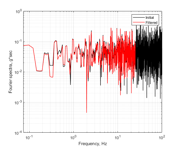
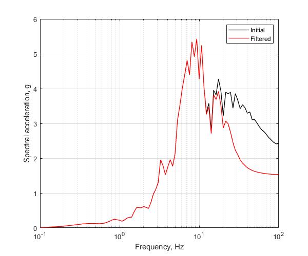
Verify Figure 3.2 of the above reference, for the the MW 6.3 Christchurch, New Zealand earthquake at Heathcote Valley Primary School (HVSC) station, Up-component. The time histories, elastic response spectra and Fourier spectra from unfiltered and filtered accelerations are shown and compared. In the above reference, the ground motion was processed following the 1970s Caltech procedure, low-pass filtered and re-sampled to 50 samples/sec by the GeoNet New Zealand strong motion network. However in this example, Butterworth filter is applied and it gives similar results.

Earthquake motion

Load earthquake data

eqmotions={'Christchurch2011HVPS_UP'};
data=load([eqmotions{1},'.dat']);
t=data(:,1);
dt=t(2)-t(1);
xgtt=data(:,2);
xgtt=[zeros(10/dt,1);xgtt];
t=(0:numel(xgtt)-1)'*dt;
xgtt=xgtt/9.81;

Apply high pass Butterworth filter

Switch

sw='butterworthhigh';

Order of Butterworth filter

bOrder=4;

Cut-off frequency

flc=0.1;

Apply OpenSeismoMatlab

S1=OpenSeismoMatlab(dt,xgtt,sw,bOrder,flc);

Filtered acceleration

cxgtt=S1.acc;

Apply low pass Butterworth filter

Switch

sw='butterworthlow';

Order of Butterworth filter

bOrder=4;

Cut-off frequency

fuc=25;

Apply OpenSeismoMatlab to high pass filtered filtered acceleration

S2=OpenSeismoMatlab(dt,cxgtt,sw,bOrder,fuc);

Filtered acceleration

cxgtt=S2.acc;

Plot the acceleration time histories

Initialize figure

figure()
hold on
plot(t,zeros(size(t)),'k','LineWidth',1)
% Plot the acceleration time history of the initial ground motion
p1=plot(t,xgtt);
% Plot the acceleration time history of the bandpass filtered ground motion
p2=plot(t,cxgtt);
% Finalize figure
hold off
grid on
legend([p1,p2],{'Initial','Filtered'})
xlabel('Time, sec')
ylabel('Acc, g')
drawnow;
pause(0.1)

Calculate the Fourier spectra

Switch

sw='fas';

Apply OpenSeismoMatlab to the initial ground motion

S3=OpenSeismoMatlab(dt,xgtt,sw);

Apply OpenSeismoMatlab to the filtered ground motion

S4=OpenSeismoMatlab(dt,cxgtt,sw);

Plot the Fourier spectra

Initialize figure

figure()
loglog(1,1,'w')
hold on
% Plot the Fourier spectrum of the initial ground motion in logarithmic
% scale for frequencies larger than 0.05 Hz
ind10=S4.freq>=0.05;
p1=loglog(S3.freq(ind10),S3.FAS(ind10),'k','LineWidth',1);
% Plot the Fourier spectrum of the filtered ground motion in logarithmic
% scale for frequencies larger than 0.05 Hz and lower than fuc
ind11=(S4.freq<=fuc)& (S4.freq>=0.05);
p2=loglog(S4.freq(ind11),S4.FAS(ind11),'r','LineWidth',1);
% Finalize figure
hold off
grid on
ylim([1e-4,1])
legend([p1,p2],{'Initial','Filtered'})
xlabel('Frequency, Hz')
ylabel('Fourier spectra, g*sec')
drawnow;
pause(0.1)

Calculate the acceleration response spectra

Switch

sw='elrs';

Critical damping ratio

ksi=0.05;
% Period range for which the response spectrum is queried
T=logspace(1,-2,100);

Apply OpenSeismoMatlab to the initial ground motion

S5=OpenSeismoMatlab(dt,xgtt,sw,T,ksi);

Apply OpenSeismoMatlab to the filtered ground motion

S6=OpenSeismoMatlab(dt,cxgtt,sw,T,ksi);

Plot the acceleration response spectra

Initialize figure

figure()
semilogx(1,1,'w')
hold on
% Plot the acceleration response spectrum of the initial ground motion in
% logarithmic scale
p1=semilogx(1./S5.Period,S5.Sa,'k','LineWidth',1);
% Plot the acceleration response spectrum of the filtered ground motion in
% logarithmic scale
p2=semilogx(1./S6.Period,S6.Sa,'r','LineWidth',1);
% Finalize figure
hold off
grid on
legend([p1,p2],{'Initial','Filtered'})
xlabel('Frequency, Hz')
ylabel('Spectral acceleration, g')
drawnow;
pause(0.1)

Copyright

Copyright (c) 2018-2023 by George Papazafeiropoulos

Published with MATLAB® R2022b